Home > Format > Conditional > Icon Sets Conditional Formatting Icon Sets Excel conditional formatting icon sets can emphasize changes up or down, indicate numbers that are good or bad, or show visual ratings or warnings, in your Excel reports and dashboards.

1.0) Conditional Formatting Icon Sets

In Excel, you can use built-in icon sets for conditional formatting. These icon sets combine colours and shapes, to give a quick visual analysis of the data.

• Tip: Download my Excel icon set examples file, to try these techniques

In this video, I show how to add an icon set to Excel data, then make quick changes to the icons. The written steps are below the video.

1.1) Numbers on the Worksheet

Here are the basic steps for applying any of the conditional formatting icon sets.

• On the worksheet shown below, there's a list of sales quantities for months January to June:
• I've selected all 6 numbers, in cells B2:B7

1.2) Start the Conditional Formatting

Next, to apply conditional formatting icons to the selected cells, I followed these steps:

• On the Excel Ribbon, click the Home tab
• In the Styles group, click the Conditional Formatting command
• Next, in the list of options, point to Icon Sets

1.3) See the Icon Sets

• In the Icon Sets menu, shown below, there are 4 types of icons:
  • 1) Directional 2) Shapes 3) Indicators 4) Ratings
• Tip: There are icon set details in the Icon Set Types section

1.4) Preview an Icon Set

If you're not sure which icon set to choose, try this:

• Point to any icon set, to see its name in a pop up tip
• On the worksheet, that icon set shows in the selected cells, as a preview

For example, in the screen shot below:

• I pointed to the 5 Arrows (Colored) icon set.
• In column B, those icons are showing, to the left of the numbers.

1.5) Choose an Icon Set

When you decide which icon set you want to use, click on that icon set in the menu

For this example, I clicked on 3 Signs. It's the second icon set in the Shapes group.

• It has the familiar traffic light colours of green, yellow and red
• It has 3 different shapes, to help anyone with vision problems

1.6) Icons on the Worksheet

On the worksheet, the 3 Shapes icon set has been applied to the selected cells.

• The original numbers are still showing in the cells
• Each cell also shows an icon, to the left of the numbers

High values have a green circle, middle values have a yellow triangle, and low values have a red diamond.

The icons make it easy to see that:

• February had the highest sales
• 3 months had low sales.

2.0) Fine Tune the Icons

When you use the Excel Ribbon commands to apply conditional formatting icon sets, Excel uses its default settings. There's a default set of icons, specific value ranges, and other settings, that you can adjust.

In the steps below, see how to:

1. Check the current icon settings
2. Make a couple of quick changes to the settings.

2.1) Check Current Icon Settings

To see the default settings for my list of 10 numbers, I followed the steps below:

• Select the cells where you applied the conditional formatting
  • Cells B2:B7 in this example
• Next, click the Conditional Formatting command, on the Excel Ribbon's Home tab
• At the bottom of the drop-down list, click on Manage Rules

2.2) Conditional Formatting Rules Manager

The Conditional Formatting Rules Manager opens.

• At the top, Current Selection was automatically entered in the "Show formatting rules for" drop down
• Below that, there is a list of rules for the selected area

To see details for a rule:

• In the list, click on the rule that you want to change.
• Next, click the Edit Rule button, to open the Edit Formatting Rule window.

2.3) Edit Formatting Rule

After you click the button, the Edit Formatting Rule window opens.

• At the top, "Format all cells based on their values" is selected.
• Do not change that setting.

Below that, in the "Edit the Rule Description" section, there are two settings that let you make a quick change to the icon sets:

• A) Reverse Icon Order
• B) Show Icon Only

2.3 A) Reverse Icon Order

If you're working with sales data, high numbers are usually good, so a green up arrow is perfect, with a red down arrow for low numbers.

However, if the data is tracking system errors, or machine down time, the opposite is true! High numbers indicate problems, and they should have a red icon.

Use the Reverse Icon Order Button

• To change the icon order, click the Reverse Icon Order button
• To return the icons to their original order, click the button again,

In the animated gif below, the green and red icons in the lower section are switched, each time I click the button.

To see the change on the worksheet:

• Click the OK button, to close the Edit Formatting Rule window.

Reverse Order Icons on Worksheet

In the screen shot below, I've added numbers in column C, to show how many items were returned each month.

For returns, a lower number is good, and higher numbers are bad for business!

I applied a 3 Signs icon set in the Returns column, and edited that rule to show a Reverse Icon Order.

• March had the highest returns, and shows a red diamond
• All other months had lower return numbers, and show green or yellow icons

2.3 B) Show Icon Only

In the Edit Formatting Rule window, the other quick setting is the Show Icon Only check box.

• ❌ To see both the numbers and the icons, leave the check box empty
• ✔️ To hide the numbers, and see only the icons, add a check mark

Icons in Formula Cells

In the screen shot below,I did something a bit different - one column has numbers only, and the next column has icons only.

• In column B, I deleted the rule for the icon set.
• Next, I added formulas in column C, linked to the numbers in the Qty column.
  • For example, in cell C2, the formula is: =B2
• I selected the formula cells (C2:C7), and applied the icon set, 3 Signs
• Next, I edited the new rule, so the formula cells show an icon only

Having the icons in a separate column lets me:

• show icons at the right, instead of the left
• control the icon position
  • I can change the cell alignment, or add an indent

3.0) Icon Set Types

There are four types of conditional formatting icon sets:

• 1) Directional 2) Shapes 3) Indicators 4) Ratings

In the sections below, I show the pop-up list from each type, and my examples of how each icon set looks on the worksheet.

3.1) Directional

First, here's the pop-up list of Directional icon sets. There are 4 sets with green, yellow and red colours, and 4 sets in grey.

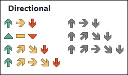
The next screen shot shows each of the directions icon sets on the worksheet.

I recommend that you use this icon set sparingly. Otherwise, the icons could make your data hard to read!

• Coloured icons: Your brain has to interpret colours, arrow directions and numbers. That's a lot to process!
• Grey icons: There are no colour cues, so you brain tries to interpret the thick arrows, that can point in 5 different directions!

3.2) Shapes

Here's the pop-up list of Shapes icon sets. There are 3 sets with green, yellow and red colours, 1 set with green, yellow, red and black, and 1 set with red, pink, grey, and black.

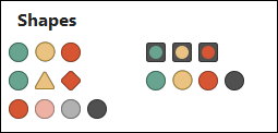
The next screen shot shows each of the shapes icon sets on the worksheet.

My choice is the 3 Signs icon set. It uses the familiar red, yellow green colours, and each colour is a different shape. That could help anyone with colour vision deficiency.

3.3) Indicators

Here's the pop-up list of Indicators icon sets. There are 3 sets with green, yellow and red colours, and 2 of the sets have familiar check marks for green and an X for red.

The next screen shot shows each of the indicator icon sets on the worksheet.

My preference is the 3 Symbols (Uncircled) icon set. It has a green check mark, a red X, and a yellow exclamation mark. Because there's no circle around them, these characters are easier to read than the 3 Symbols (circled)

3.4) Ratings

Here's the pop-up list of Ratings icon sets. There are 5 sets, with stars, circles, squares, and bars. Each set has only 2 colours - yellow and white, or black and white, or blue and grey.

The next screen shot shows each of the ratings icon sets on the worksheet.

My preference is the 3 Stars icon set. It's the simplest set, and easiest to interpret at a quick glance. The other sets are more complicated, and could distract from the data.

4.0) Cell Alignment with Icons

When you add icon sets to worksheet cells, the cell alignment might not work exactly as you expect!

In the screen shot below, there are cells with numbers and icons, and cells with icons only. I formatted the cells with four types of horizontal alignment:

• 1) Center   2) Right   3) Left   4) Left with Indent

For cells with numbers and icons:

• Icons are always at the left border
• Numbers adjust to the selected cell alignment

For cells icons only:

• Icons adjust to the selected cell alignment

5.0) Column Width Problem with Icons

When you use icon sets in number cells, the Excel column autofit feature doesn't work correctly in all cases.

• Numbers and Icons: After Autofit, numbers might overlap the icons
• Icons Only: Autofit has no effect on these cells - they stay at their current width

To avoid these column width problems, I recommend that you manually adjust the column widths, if possible.

6.0) Get the Excel File ✅

• Icon Sets: Get the icon set examples file. The zipped Excel file is in xlsx format, and does not contain any macros.

Get Monthly Excel Tips!

Don't miss my monthly Excel newsletter! You'll get quick tips, article links, and a bit of fun. Add your email, and click Sign Up.

Next, when you get my reply, click the Confirm button. I add this step to protect you from spam!

More Tutorials

Conditional Formatting Intro

Conditional Formatting Examples

Custom Icon Sets

Conditional Format Color Scales

Fix Conditional Formatting Extra Rules

Conditional Formatting Multiple Cells

Conditional Formatting - Currency

Conditional Formatting Documentation

Conditional Formatting Data Bars