Home > Formulas > Functions > Compare Compare Cell Values in Excel-Troubleshoot In Excel compare two cells, to test for an exact match or partial match. Cell values can look equal, but have hidden differences. Troubleshoot VLOOKUP formula errors

1) Compare Cell Values in Excel

Sometimes in Excel, two cell values look the same, but Excel sees them as different.

In the examples below, there are simple formulas to compare cells, and tougher formulas:

• First, I show a few quick ways to compare cell values, to see if they're equal.
• After that, I compare cells for partial matches, using fancier formulas.

2) Quick Tests to Compare Two Cells

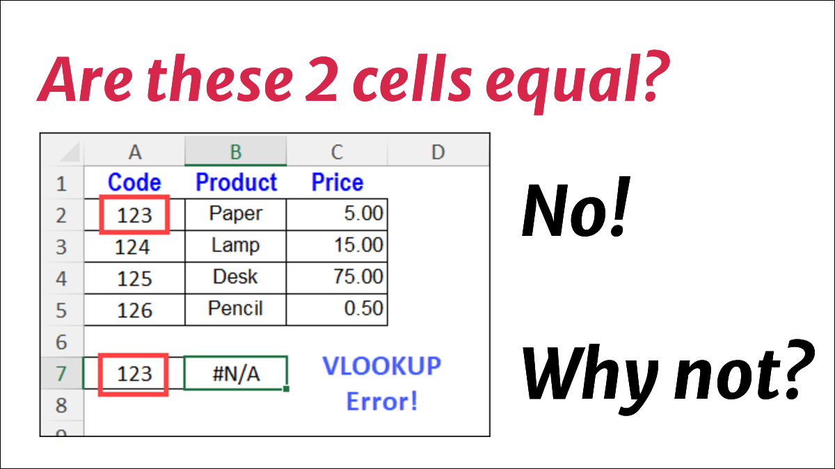
In the screen shot below, two cell values look the same (123).

• ✅  To follow along, get the Compare Cells sample file.

But my VLOOKUP formula shows an #N/A error, because Excel can't find 123 in the little product lookup table.

In the examples below, I use 3 quick tests to compare cells A2 and A7. Why does Excel see them as different.

• Test A: Compare With Equal Sign
• Test B: Compare Cell Values Length
• Test C: Compare Cell Data Type
• TestD: Compare Cell Including Case

2.1) Test A: Compare With Equal Sign

For the simplest test, I use the equal sign in a formula, to compare the two cells.

In the screen shot below, I put the following formula in cell A9:

• =A2=A7

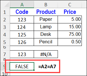
The result of that formula is FALSE - the cell values are NOT equal.

• Note: For text values, upper and lower case letters are treated as equal

2.2) Test B: Compare Cell Values Length

For another quick test, I'll use the Excel LEN function, to see if the two cell values are the same length.

• There could be extra spaces in a cell, at the start, the end, or between words.

I entered the following LEN formulas, to compare the lengths:

• Cell A9:   =LEN(A2)
• Cell B9:   =LEN(A7)

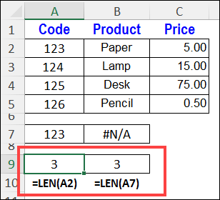
The result for both formulas is 3, so there are no hidden characters in either cell.

Formula Fix - Extra Spaces

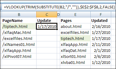
To fix a VLOOKUP formula, so it will ignore extra spaces, you can use the TRIM function inside the VLOOKUP. For detailed step, see this VLOOKUP example on my Contextures Blog.

In the screen shot below, the VLOOKUP formula includes TRIM, to remove extra spaces, and SUBSTITUTE, to remove the leading slash character, in the lookup value.

2.3) Test C: Compare Cell Data Type

For my third test, I'll use the ISNUMBER function, to see if the two cell values are real numbers. Sometimes cells contain "text" numbers, instead of real numbers, especially if the data was imported, or copied from a website.

To check, I entered the following formulas, to test for numberss:

• Cell A9:   =ISNUMBER(A2)
• Cell B9:   =ISNUMBER(A7)

The results for the above formulas show that the:

• value in cell A2 is NOT a real number
• value in cell A7 IS a real number.

A real number is not a match for a text number. That's why Excel couldn't find matching data for product code 123 (real number) in the lookup table, and returned an #NA error.

Formula Fix - Real Numbers and Text Numbers

In the video below, I show how to change a VLOOKUP formula, so it will fix the mismatched data problem of real numbers vs text numbers. There are written steps on the VLOOKUP Examples page.

Video: VLOOKUP Formula Fix

To see the steps for fixing VLOOKUP formula when the lookup table has text numbers that cause a mismatch, watch this short video. There are written steps on the VLOOKUP Examples page.

Video Timeline

• 00:00 VLOOKUP Error Problem
• 00:44 Values Not Equal
• 01:37 Fix Values Not Equal
• 02:07 Change VLOOKUP Formula

2.4) Test D: Compare Cells Including Case

If you need to compare two cells for contents, including a case sensitive comparison of letters, use the Excel EXACT function.

In the password example below, the EXACT function compares two cells, including UPPER and lower case.

• =EXACT(A2,B2)

The EXACT function result is FALSE, because cell A2 has lower case and cell B2 has upper case.

• Note: EXACT function does NOT compare the cell formatting, like bold or italic.

2.4.1) Video: EXACT Function Examples

This video shows a few more EXACT function examples. For each example shown in the video, you'll find the written steps for each example on the EXACT Function Examples page. You can download the sample file there too.

3) Partially Compare Two Cells

Sometimes you don’t need a full comparison of two cells – you just need to check the first few characters at the left, or a 3-digit code at the right end of a string.

The following examples use the LEFT and RIGHT functions to compare partial text in two different cells.

3.1) Compare from Left

To compare characters at the beginning of the cells, use the LEFT function. For example, check the first 3 characters:

• =LEFT(A2,3)=LEFT(B2,3)

3.2) Compare from Right

To compare characters at the end of the cells, use the RIGHT function. For example, check the last 3 characters:

• =RIGHT(A2,3)=RIGHT(B2,3)

3.3) Ignore Extra Space Characters

You can combine LEFT or RIGHT with TRIM, if you’re not concerned about the space characters:

• =RIGHT(TRIM(A2),3)=RIGHT(TRIM(B2),3)

And combine LEFT or RIGHT with EXACT, to check if upper/lower case match too. This formula will ignore extra spaces, but checks the case:

• =EXACT(RIGHT(TRIM(A2),3),RIGHT(TRIM(B2),3))

4) Find Percent 2 Cells Match

Finally, here’s an advanced Excel formula that compares old and new addresses.

Starting from the left of each cell, what percent match is there?

In the screen shot below, there’s a small sample list:

• Old addresses are in column A
• New addresses are in column B
• Formulas in columns C, D and E compare the addresses

Thanks to UniMord, who contributed this example.

4.1) Percent Match Formulas

Here's what the 3 formulas do, and the formula details are shown in the sections below:

1. Col C: Calculate length of text in column A.
2. Col D: For that number of characters, how many characters in column B are a match, starting from the left?
3. Col E: Compare results from first two formulas, to calculate the percent match

4.2) Col C: Get Text Length

The first step is to find the length of the old address in column A. This formula is in cell C2, and copied down:

• =LEN(A2)

4.3) Col D: Get Match Length

The formula in column D does the hard work. It finds how many characters, starting from the left in each cell, are a match. Lower and upper case are not compared.

• Note: There are 2 formulas shown below-- one for Excel 365, and one for earlier versions of Excel

A) For Excel 365, or other versions that have the new Spill Functions, use this formula:

• =SUMPRODUCT(--(LEFT(A2, SEQUENCE(C2))
  =LEFT(B2,SEQUENCE(C2))))

B) For earlier versions of Excel, use this formula -- it will work in any version of Excel:

• =SUMPRODUCT( –(LEFT(A2, ROW(INDIRECT(“A1:A” & C2)))
  =LEFT(B2, ROW(INDIRECT(“A1:A” &C2)))))

4.3.1) How the Formulas Work

The example in the screen shot below shows a summary of the steps.

1. Get the characters from the left of each cell
2. Compare the characters, to see if they are equal
3. Convert TRUE and FALSE to 1 and 0
4. Get a sum of the 1s and 0s

For more details on how these two Match Length formulas work, go to the How Match Len Formula Works section below.

4.4) Col E: Get the Percent Match

Once the text length and the match length have been calculated, it just takes a simple formula to find the percent matched.

Here is the result column formula from cell E2, to compare the two lengths:

• =D2/C2

There is a 100% match in row 2, and only a 20% match, starting from the left, in row 5.

4.5) How Match Len Formula Works

• Note: You can skip reading this section, unless you want more details on how the Match Length formulas work.

In column D, the Match Len formula compares the 2 cells, to see how many characters match, starting from the left. To get the result, the formula does 4 things:

1. Get X cell characters, starting from the LEFT of each cell
• Functions create an array of numbers, for the LEFT function to use
2. Compare character strings, to see if they are equal - TRUE or FALSE
3. Change TRUE and FALSE to numbers (one and zero)
4. Add up the ones and zeros, to get the total number of matching characters

4.5.1) Get Cell Characters

To find out how many characters have an equal match, the formula will use the LEFT function to:

• get characters from the two cells
• start from the left
• start with 1 character, and go to X characters

Usually, we enter a single numbers as the second argument for the LEFT function. However, for this formula, we want the LEFT function to check a list of numbers, from 1 to X.

If we typed the list of numbers in the formula, the numbers would be in an array, like this:

• =LEFT(A2,{1;2;3;4;5;6;7;8;9}) = LEFT(B2,{1;2;3;4;5;6;7;8;9})

4.5.2) Create Array of Numbers with Formula

We don't want to type an array of numbers into the formula though. We want Excel to automatically create a list of numbers, starting with 1, and ending at X. (X is the length of Address01, in this example)

There are two formulas shown below, so use that one that works in your version of Excel:

4.5.3) Array of Numbers - Excel 365

Use this shorter formula, in Excel 365, or other versions that have the new Spill Functions. In it, the SEQUENCE function creates the list of numbers:

• =SUMPRODUCT(--(LEFT(A2, SEQUENCE(C2))
  =LEFT(B2, SEQUENCE(C2))))

4.5.4) Array of Numbers - All Versions of Excel

For earlier versions of Excel, use this longer formula. It will work in any version of Excel, and uses two functions to create the list of numbers - ROW and INDIRECT:

• =SUMPRODUCT( –(LEFT(A2, ROW(INDIRECT(“A1:A” & C2)))
  =LEFT(B2, ROW(INDIRECT(“A1:A” & C2)))))

Here's how the ROW and INDIRECT functions work together, to create the list of numbers:

• First, the INDIRECT function creates a reference to a range of cells -- “A1:A” & C2
  • In row 2, that calculates to “A1:A9”
• Next, the ROW function returns an array, with the row number for each cell in that range;
  • In row 2, that array is {1;2;3;4;5;6;7;8;9}

In the screen shot below, you can see the list of numbers that the two functions create. To make that list appear, follow these steps:

4.5.5) Are Cell Character Strings Equal?

After the LEFT function gets character strings from each cell, the equal sign compares those stings.

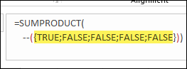
• The result from each comparison is TRUE (equal) or FALSE (not equal)

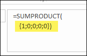
In the screen shot below, there were 5 character strings to compare. The first result is TRUE, and the remaining four results are FALSE.

4.5.6) Change TRUE and FALSE to Numbers

Next, the double minus sign, near the start of the formula, converts:

• each TRUE to a 1 (one)
• each FALSE to a 0 (zero)

4.5.7) Add the Numbers

Finally, the SUMPRODUCT function adds up those numbers, to calculate the total number of characters, from the left, that match.

In cell D5, in the screen shot below, the total is 1.

• Starting from the left in cells A5 and B5, only 1 character was a match.

Get the Excel Files ✅

• Compare Cells: Download the sample file with Compare Cells examples from this tutorial. The zipped Excel file is in xlsx format, and does not contain macros.

Get Monthly Excel Tips!

Don't miss my monthly Excel newsletter! You'll get quick tips, article links, and a bit of fun. Add your email, and click Sign Up.

Next, when you get my reply, click the Confirm button. I add this step to protect you from spam!

More Ways to Compare Two Cells

Here are a few more articles that show examples of how to compare two cells – either the full content, or partial content.

1. How to troubleshoot and fix VLOOKUP problems for lookup numbers that don't match
2. Use INDEX, MATCH and COUNTIF to find codes within text strings. There are other formulas in the comments too, so check those out.
3. Compare formulas on different sheets, with the FORMULATEXT and INDIRECT functions. Those functions are volatile though, so they’d slow down the workbook if you use too many of them.
4. Be careful when using the Remove Duplicates feature in Excel – it treats real numbers and text numbers as the same value

 

Related Tutorials

Compare 2 Lists

SUMPRODUCT function

SEQUENCE function

INDEX / MATCH Functions

INDIRECT function

EXACT Function Examples

VLOOKUP Troubleshooting

VLOOKUP Examples

Excel Spill Functions