Home > Formulas > Statistical > RANK Excel RANK With Ties How to handle Excel rank with ties. Show all ties at same rank, or break any ties, if needed. For contests, split winnings for tied scores. Watch the videos, and get the free RANK workbook

1) Break Ties With RANK Function

In some cases, ties aren't allowed, so you have to find a way to break the tie.

Watch this video to see the steps, and the written instructions are below the video.

• ✅  To follow along, get the Excel file in the download section

Tip: To get started with RANK, go to the RANK Function Examples page

1.1) Break Ties With RANK Function

In the video above, I kept track of how many minutes each student worked on the test. That time is in the scores list, and I use that time to break any ties.

If scores are tied, the student who takes less time to complete the test will rank ahead of the other student with the same score.

1.2) Calculate Decimal Amount for Tied Scores

In the screen shot below, Test Times are in column C, and a TieBreak formula is in in column E.

Here's the formula in cell E2, and it refers the the score (B2) and time (C2) in row 2:

• =IF(COUNTIF($B$2:$B$11,B2)>1,
         RANK(C2,$C$2:$C$11,1)/100,0)

1.3) How Tiebreaker Formula Works

In column E, the Tie Break formula uses COUNTIF and RANK functions, wrapped with an IF function, to see if a tie-breaking decimal amount should be added to the original Rank.

1. First, the TieBreak formula checks to see IF there is more than one instance of the score number in the entire list:
      IF(COUNTIF($B$2:$B$11,B2)>1
2. If there is more than one instance, it ranks the Times in ascending order, because a lower time is better, :
• RANK(C2,$C$2:$C$11,1)
• The 3rd argument (order) is 1 -- ascending (smallest to largest)
3. Next, the formula divides that amount by 100, to get a decimal amount. .
• /100
• Note: The divisor, 100, could be changed to another number, if you are working with a longer list.
• Later, you'll add this decimal amount to the original Rank
  
4. Finally, to complete the IF function, if there is only one instance of a Rank, the result for the TieBreak is zero.
   •  ,0)

1.4) Calculate the Final Rank

After calculating the tie-breaking decimal amounts, you can add the RANK function results to the TieBreak results, to get the final ranking.

In this example, two students were tied in 4th place.

• Joe finished the test in 27 minutes, and his Time was ranked 5th.
• Ivy finished the test in 29 minutes, and her Time was ranked 9th.

The Tie Break formula adds a decimal of 0.09 to Ivy's score, and 0.05 to Joe's score.

In the final ranking, Joe, with 4.05, ranks higher than Ivy, with 4.09.

2) Split Winnings for Tied Rank

In a tournament, instead of breaking the ties, you might want to split the winnings among any tied players, if you're awarding a cash prize, or points.

To see the steps for splitting the winnings, watch this short video. The written instructions are below the video.

• ✅  To follow along, get the Excel sample file in the download section

2.1) Split Winnings for Tied Rank

In this example, there is a list, with ranks from 1 to 10, and the prize amount for each rank.

If two or more players are tied in the rankings, the prize amounts are pooled, and then split equally among the tied players.

In this example, if 3 players are at rank 1, they would split the total amount (10+9+8=27) for ranks 1, 2 and 3.

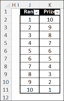
• Each of the 3 players at rank 1 earns 9 (27/3 = 9)
• The player with the next best score would be ranked 4th, and earn 7.

2.2) Calculate the Split Amount

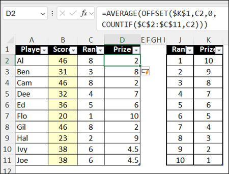
To split the prize amount among tied players, there is a Prize formula in column D.

The formula uses the AVERAGE function, with the OFFSET function finding the range of cells to average.

This formula is entered in cell D2 and copied down to cell D11.

• =AVERAGE(OFFSET($K$1,C2,0, COUNTIF($C$2:$C$11,C2)))

2.3) How the Prize Formula Works

The Prize formula uses the AVERAGE function, with the OFFSET function finding the range of cells to average.

• =AVERAGE(OFFSET($K$1,C2,0, COUNTIF($C$2:$C$11,C2)))

2.3.1) Find the Prize Range

To find the range of prize amount cells, this OFFSET function has 4 arguments:

1. reference: starting point
2. rows: rows to move from starting point
3. cols: columns to move from starting point
4. height: number of rows to include

To get the prize amount range, the formula uses these settings for the arguments:

1. reference: $K$1 - heading cell for prize column
2. rows: C2 - player's rank - where to start the prize range
3. cols:  0 - move zero columns
4. height:  COUNTIF($C$2:$C$11,C2) - count of players with the same score

2.3.2) Find the Average

After the prize amount range is returned by the OFFSET function, the AVERAGE function returns the average for the numbers in that range.

3) Get the Excel Files ✅

Rank Tied: Click here to get a zipped sample RANK With Ties Excel file with the examples from this tutorial. The zipped workbook is in xlsx format, and there are no macros in the file.

Get Monthly Excel Tips!

Don't miss my monthly Excel newsletter! You'll get quick tips, article links, and a bit of fun. Add your email, and click Sign Up.

Next, when you get my reply, click the Confirm button. I add this step to protect you from spam!

Related Links

RANK Function Examples

XLOOKUP

AVERAGE

COUNT / COUNTIF

MIN / MAX

SUM / SUMIF